Note
Click here to download the full example code
Linear regression
We are going to look at the relationship between age and minutes played. Start by watching the video a
Either work through the code at the same time as watching or afterwards.
#importing necessary libraries
import pandas as pd
import numpy as np
import matplotlib.pyplot as plt
import statsmodels.formula.api as smf
Opening data
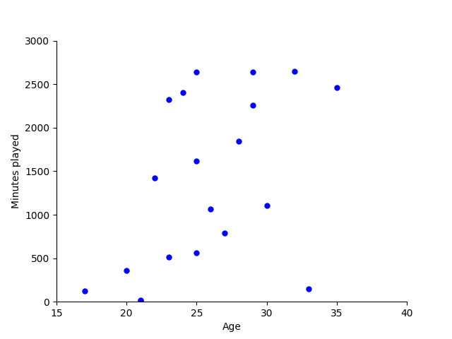
In this example we use data downloaded from FBref on players in La Liga. We just use the age and minutes played columns. And we only take the first 20 observations, to help visualise the process. Download playerstats.csv your working directory.
num_obs=20
laliga_df=pd.read_csv("playerstats.csv",delimiter=',')
minutes_model = pd.DataFrame()
minutes_model = minutes_model.assign(minutes=laliga_df['Min'][0:num_obs])
minutes_model = minutes_model.assign(age=laliga_df['Age'][0:num_obs])

# Make an age squared column so we can fir polynomial model.
minutes_model = minutes_model.assign(age_squared=np.power(laliga_df['Age'][0:num_obs],2))
Plotting the data
Start by plotting the data.
fig,ax=plt.subplots(num=1)
ax.plot(minutes_model['age'], minutes_model['minutes'], linestyle='none', marker= '.', markersize= 10, color='blue')
ax.set_ylabel('Minutes played')
ax.set_xlabel('Age')
ax.spines['top'].set_visible(False)
ax.spines['right'].set_visible(False)
plt.xlim((15,40))
plt.ylim((0,3000))
plt.show()
Fitting the model
- We are going to begin by doing a straight line linear regression
- \[y = b_0 + b_1 x\]
A straight line relationship between minutes played and age.
model_fit=smf.ols(formula='minutes  ~ age   ', data=minutes_model).fit()
print(model_fit.summary())
b=model_fit.params
                            OLS Regression Results
==============================================================================
Dep. Variable:                minutes   R-squared:                       0.231
Model:                            OLS   Adj. R-squared:                  0.189
Method:                 Least Squares   F-statistic:                     5.415
Date:                Wed, 24 Apr 2024   Prob (F-statistic):             0.0318
Time:                        18:38:00   Log-Likelihood:                -163.24
No. Observations:                  20   AIC:                             330.5
Df Residuals:                      18   BIC:                             332.5
Df Model:                           1
Covariance Type:            nonrobust
==============================================================================
                 coef    std err          t      P>|t|      [0.025      0.975]
------------------------------------------------------------------------------
Intercept  -1293.0147   1152.158     -1.122      0.277   -3713.609    1127.580
age          102.5404     44.065      2.327      0.032       9.963     195.118
==============================================================================
Omnibus:                        0.142   Durbin-Watson:                   2.001
Prob(Omnibus):                  0.931   Jarque-Bera (JB):                0.316
Skew:                          -0.153   Prob(JB):                        0.854
Kurtosis:                       2.466   Cond. No.                         151.
==============================================================================

Notes:
[1] Standard Errors assume that the covariance matrix of the errors is correctly specified.
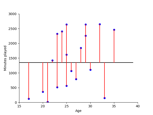
- Comparing the fit
- We now use the fit to plot a line through the data.
- \[y = b_0 + b_1 x\]
where the parameters are estimated from the model fit.
#First plot the data as previously
fig,ax=plt.subplots(num=1)
ax.plot(minutes_model['age'], minutes_model['minutes'], linestyle='none', marker= '.', markersize= 10, color='blue')
ax.set_ylabel('Minutes played')
ax.set_xlabel('Age')
ax.spines['top'].set_visible(False)
ax.spines['right'].set_visible(False)
plt.xlim((15,40))
plt.ylim((0,3000))

#Now create the line through the data
x=np.arange(40,step=1)
y= np.mean(minutes_model['minutes'])*np.ones(40)
ax.plot(x, y, color='black')

#Show distances to line for each point
for i,a in enumerate(minutes_model['age']):
    ax.plot([a,a],[minutes_model['minutes'][i], np.mean(minutes_model['minutes']) ], color='red')
plt.show()
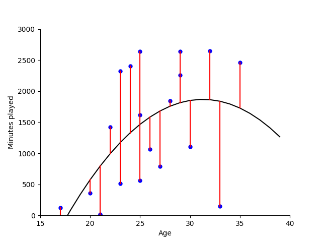
- A model including squared terms
- We now fit the quadratic model
- \[y = b_0 + b_1 x + b_2 x^2\]
estimating the parameters from the data.
# First fit the model
model_fit=smf.ols(formula='minutes  ~ age + age_squared  ', data=minutes_model).fit()
print(model_fit.summary())
b=model_fit.params

# Compare the fit
fig,ax=plt.subplots(num=1)
ax.plot(minutes_model['age'], minutes_model['minutes'], linestyle='none', marker= '.', markersize= 10, color='blue')
ax.set_ylabel('Minutes played')
ax.set_xlabel('Age')
ax.spines['top'].set_visible(False)
ax.spines['right'].set_visible(False)
plt.xlim((15,40))
plt.ylim((0,3000))
x=np.arange(40,step=1)
y= b[0] + b[1]*x + b[2]*x*x
ax.plot(x, y, color='black')

for i,a in enumerate(minutes_model['age']):
    ax.plot([a,a],[minutes_model['minutes'][i], b[0] + b[1]*a + b[2]*a*a], color='red')
plt.show()
                            OLS Regression Results
==============================================================================
Dep. Variable:                minutes   R-squared:                       0.295
Model:                            OLS   Adj. R-squared:                  0.212
Method:                 Least Squares   F-statistic:                     3.559
Date:                Wed, 24 Apr 2024   Prob (F-statistic):             0.0512
Time:                        18:38:00   Log-Likelihood:                -162.38
No. Observations:                  20   AIC:                             330.8
Df Residuals:                      17   BIC:                             333.7
Df Model:                           2
Covariance Type:            nonrobust
===============================================================================
                  coef    std err          t      P>|t|      [0.025      0.975]
-------------------------------------------------------------------------------
Intercept   -8063.5823   5573.188     -1.447      0.166   -1.98e+04    3694.817
age           634.7722    431.113      1.472      0.159    -274.796    1544.340
age_squared   -10.1432      8.174     -1.241      0.232     -27.389       7.103
==============================================================================
Omnibus:                        1.800   Durbin-Watson:                   2.164
Prob(Omnibus):                  0.407   Jarque-Bera (JB):                1.054
Skew:                          -0.190   Prob(JB):                        0.590
Kurtosis:                       1.942   Cond. No.                     2.06e+04
==============================================================================

Notes:
[1] Standard Errors assume that the covariance matrix of the errors is correctly specified.
[2] The condition number is large, 2.06e+04. This might indicate that there are
strong multicollinearity or other numerical problems.
Now try with all data points
Refit the model with all data points
Try adding a cubic term
Think about how well the model works. What are the limitations?
Total running time of the script: ( 0 minutes 0.380 seconds)