Note
Click here to download the full example code
Fitting the xG model
In this page we go through all the steps of statistically fitting an expected goals model.
Before starting watch the following two videos from Friends of Tracking.
You will be sad to learn that Tobias (the dog featuring in this video) died suddenly during summer 2022 :-(
These use an older version of the code, which is available here. But the steps are the same.
# importing necessary libraries
import pandas as pd
import numpy as np
import json
# plotting
import matplotlib.pyplot as plt
from mplsoccer import VerticalPitch
# statistical fitting of models
import statsmodels.api as sm
import statsmodels.formula.api as smf
#opening data
import os
import pathlib
import warnings

pd.options.mode.chained_assignment = None
warnings.filterwarnings('ignore')
Opening data
To fit the xG model we will use Wyscout data. To meet file size requirements of Github, we have to open it from different files, but you can open the file locally from the directory you saved it in.
#load data - store it in train dataframe
train = pd.DataFrame()
for i in range(13):
    file_name = 'events_England_' + str(i+1) + '.json'
    path = os.path.join(str(pathlib.Path().resolve().parents[0]), 'data', 'Wyscout', file_name)
    with open(path) as f:
        data = json.load(f)
    train = pd.concat([train, pd.DataFrame(data)])
Preparing data
Exepcted goals model is build using only shots, so we keep only those actions which subEventName was Shot. Note that this way penalties are excluded which wouldn’t be a case if we used only eventName. Then, we store the coordinates of a shot transformed to 105 x 68 pitch. Also, we treat the goal as x = 0. Created C is an auxillary variable to help us calculate distance and angle. It is the distance from a point to the horizontal line through the middle of the pitch. We calculate the distance to the goal as the distance on Euclidean plane (see Distance in R2). and angle using the formula from The Geometry of Shooting. Moreover, we need an information if a goal was scored. It can be found in the tags column - if in this column exists {id: 101}.
shots = train.loc[train['subEventName'] == 'Shot']
#get shot coordinates as separate columns
shots["X"] = shots.positions.apply(lambda cell: (100 - cell[0]['x']) * 105/100)
shots["Y"] = shots.positions.apply(lambda cell: cell[0]['y'] * 68/100)
shots["C"] = shots.positions.apply(lambda cell: abs(cell[0]['y'] - 50) * 68/100)
#calculate distance and angle
shots["Distance"] = np.sqrt(shots["X"]**2 + shots["C"]**2)
shots["Angle"] = np.where(np.arctan(7.32 * shots["X"] / (shots["X"]**2 + shots["C"]**2 - (7.32/2)**2)) > 0, np.arctan(7.32 * shots["X"] /(shots["X"]**2 + shots["C"]**2 - (7.32/2)**2)), np.arctan(7.32 * shots["X"] /(shots["X"]**2 + shots["C"]**2 - (7.32/2)**2)) + np.pi)
#if you ever encounter problems (like you have seen that model treats 0 as 1 and 1 as 0) while modelling - change the dependant variable to object
shots["Goal"] = shots.tags.apply(lambda x: 1 if {'id':101} in x else 0)
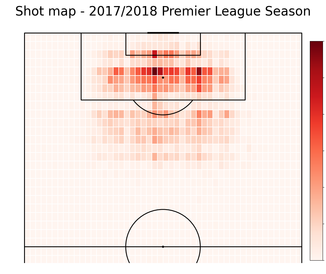
Plotting shot location
Since we would like to investigate the relationship between shot location and goal location, first we create a heat map of all shots from the 2017/18 Premier League season.
#plot pitch
pitch = VerticalPitch(line_color='black', half = True, pitch_type='custom', pitch_length=105, pitch_width=68, line_zorder = 2)
fig, ax = pitch.grid(grid_height=0.9, title_height=0.06, axis=False,
                     endnote_height=0.04, title_space=0, endnote_space=0)
#subtracting x from 105 but not y from 68 because of inverted Wyscout axis
#calculate number of shots in each bin
bin_statistic_shots = pitch.bin_statistic(105 - shots.X, shots.Y, bins=50)
#make heatmap
pcm = pitch.heatmap(bin_statistic_shots, ax=ax["pitch"], cmap='Reds', edgecolor='white', linewidth = 0.01)
#make legend
ax_cbar = fig.add_axes((0.95, 0.05, 0.04, 0.8))
cbar = plt.colorbar(pcm, cax=ax_cbar)
fig.suptitle('Shot map - 2017/2018 Premier League Season' , fontsize = 30)
plt.show()
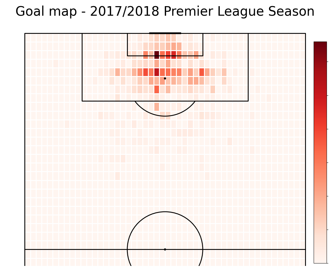
Plotting goal location
Having the shot location, we would also like to know where the goals were scored from.
#take only goals
goals = shots.loc[shots["Goal"] == 1]
#plot pitch
pitch = VerticalPitch(line_color='black', half = True, pitch_type='custom', pitch_length=105, pitch_width=68, line_zorder = 2)
fig, ax = pitch.grid(grid_height=0.9, title_height=0.06, axis=False,
                     endnote_height=0.04, title_space=0, endnote_space=0)
#calculate number of goals in each bin
bin_statistic_goals = pitch.bin_statistic(105 - goals.X, goals.Y, bins=50)
#plot heatmap
pcm = pitch.heatmap(bin_statistic_goals, ax=ax["pitch"], cmap='Reds', edgecolor='white')
#make legend
ax_cbar = fig.add_axes((0.95, 0.05, 0.04, 0.8))
cbar = plt.colorbar(pcm, cax=ax_cbar)
fig.suptitle('Goal map - 2017/2018 Premier League Season' , fontsize = 30)
plt.show()
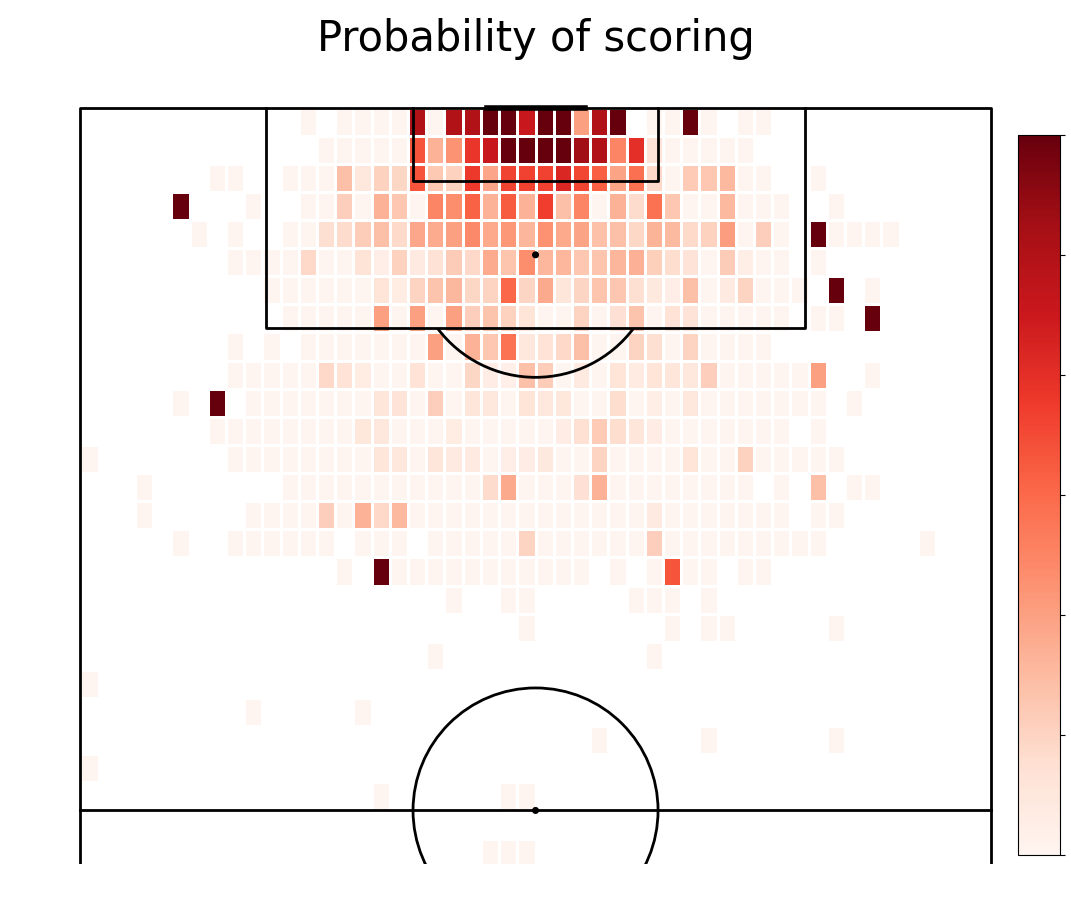
Plotting the probability of scoring a goal given the location
Now, we can calculate the proportion of goals scored from each bin to number of shots from that location.
#plot pitch
pitch = VerticalPitch(line_color='black', half = True, pitch_type='custom', pitch_length=105, pitch_width=68, line_zorder = 2)
fig, ax = pitch.grid(grid_height=0.9, title_height=0.06, axis=False,
                     endnote_height=0.04, title_space=0, endnote_space=0)
bin_statistic = pitch.bin_statistic(105 - shots.X, shots.Y, bins = 50)
#normalize number of goals by number of shots
bin_statistic["statistic"] = bin_statistic_goals["statistic"]/bin_statistic["statistic"]
#plot heatmap
pcm = pitch.heatmap(bin_statistic, ax=ax["pitch"], cmap='Reds', edgecolor='white', vmin = 0, vmax = 0.6)
#make legend
ax_cbar = fig.add_axes((0.95, 0.05, 0.04, 0.8))
cbar = plt.colorbar(pcm, cax=ax_cbar)
fig.suptitle('Probability of scoring' , fontsize = 30)
plt.show()
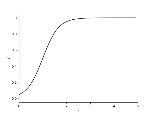
Plotting a logistic curve
Plotting logistic curve
b = [3, -3]
x = np.arange(5, step=0.1)
y = 1/(1+np.exp(b[0]+b[1]*x))
fig,ax = plt.subplots()
plt.ylim((-0.05,1.05))
plt.xlim((0,5))
ax.set_ylabel('y')
ax.set_xlabel("x")
ax.plot(x, y, linestyle='solid', color='black')
ax.spines['top'].set_visible(False)
ax.spines['right'].set_visible(False)
plt.show()
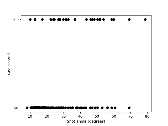
Investigating the relationship between goals and angle
We want to find out if the angle influences scoring a goal. First we plot if goal was scored given the angle.
#first 200 shots
shots_200=shots.iloc[:200]
#plot first 200 shots goal angle
fig, ax = plt.subplots()
ax.plot(shots_200['Angle']*180/np.pi, shots_200['Goal'], linestyle='none', marker= '.', markersize= 12, color='black')
#make legend
ax.set_ylabel('Goal scored')
ax.set_xlabel("Shot angle (degrees)")
plt.ylim((-0.05,1.05))
ax.set_yticks([0,1])
ax.set_yticklabels(['No','Yes'])
plt.show()
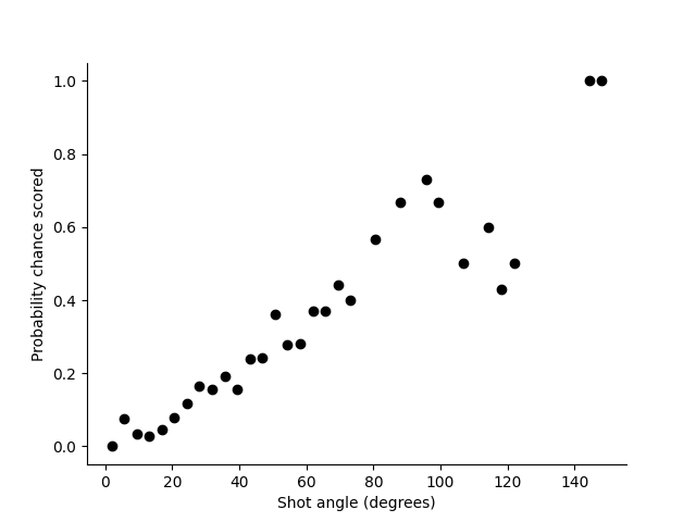
Investigating the relationship between probability of scoring goals and angle
We want to find out if the angle influences the probability of scoring a goal. First we plot if goal was scored given the angle.
#number of shots from angle
shotcount_dist = np.histogram(shots['Angle']*180/np.pi, bins=40, range=[0, 150])
#number of goals from angle
goalcount_dist = np.histogram(goals['Angle']*180/np.pi, bins=40, range=[0, 150])
np.seterr(divide='ignore', invalid='ignore') #Ignore divide by 0
#probability of scoring goal
prob_goal = np.divide(goalcount_dist[0], shotcount_dist[0])
angle = shotcount_dist[1]
#Midangle of each interval
midangle = (angle[:-1] + angle[1:])/2
#make plot
fig,ax = plt.subplots()
ax.plot(midangle, prob_goal, linestyle='none', marker= '.', markersize= 12, color='black')
ax.set_ylabel('Probability chance scored')
ax.set_xlabel("Shot angle (degrees)")
ax.spines['top'].set_visible(False)
ax.spines['right'].set_visible(False)
plt.show()
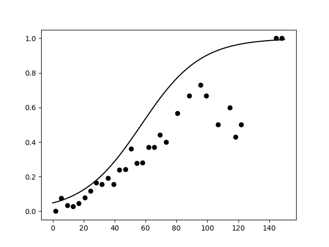
Fitting logistic regression with random coefficients
To our data we fit a logistic regression curve with set parameters; -3 for intercept and 3 for angle. However, these are most likely not the best estimators of true parameters.
fig, ax = plt.subplots()
b = [-3, 3]
x = np.arange(150,step=0.1)
y = 1/(1+np.exp(-(b[0]+b[1]*x*np.pi/180)))
#plot line
ax.plot(midangle, prob_goal, linestyle='none', marker= '.', markersize= 12, color='black')
#plot logistic function
ax.plot(x, y, linestyle='solid', color='black')
ax.set_ylabel('Probability chance scored')
ax.set_xlabel("Shot angle (degrees)")
ax.spines['top'].set_visible(False)
ax.spines['right'].set_visible(False)
plt.show()
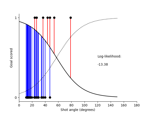
Calculating log-likelihood
The best parameters are those which maximize the log-likelihood.
#calculate xG
xG = 1/(1+np.exp(-(b[0]+b[1]*shots['Angle'])))
shots = shots.assign(xG = xG)
shots_40 = shots.iloc[:40]
fig, ax = plt.subplots()
#plot data
ax.plot(shots_40['Angle']*180/np.pi, shots_40['Goal'], linestyle='none', marker= '.', markersize= 12, color='black', zorder = 3)
#plot curves
ax.plot(x, y, linestyle=':', color='black', zorder = 2)
ax.plot(x, 1-y, linestyle='solid', color='black', zorder = 2)
#calculate loglikelihood
loglikelihood=0
for item,shot in shots_40.iterrows():
    ang = shot['Angle'] * 180/np.pi
    if shot['Goal'] == 1:
        loglikelihood = loglikelihood + np.log(shot['xG'])
        ax.plot([ang,ang],[shot['Goal'],1-shot['xG']], color='red', zorder = 1)
    else:
        loglikelihood = loglikelihood + np.log(1 - shot['xG'])
        ax.plot([ang,ang], [shot['Goal'], 1-shot['xG']], color='blue', zorder = 1)
#make legend
ax.set_ylabel('Goal scored')
ax.set_xlabel("Shot angle (degrees)")
plt.ylim((-0.05,1.05))
plt.xlim((0,180))
plt.text(120,0.5,'Log-likelihood:')
plt.text(120,0.4,str(loglikelihood)[:6])
ax.set_yticks([0,1])
ax.spines['top'].set_visible(False)
ax.spines['right'].set_visible(False)
plt.show()
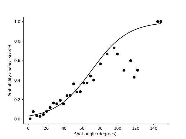
Fitting logistic regression and finding best parameters
The best parameters are those which maximize the log-likelihood.
#create model
test_model = smf.glm(formula="Goal ~ Angle" , data=shots,
                           family=sm.families.Binomial()).fit()
print(test_model.summary())
#get params
b=test_model.params
#calculate xG
xGprob = 1/(1+np.exp(-(b[0]+b[1]*midangle*np.pi/180)))
fig, ax = plt.subplots()
#plot data
ax.plot(midangle, prob_goal, linestyle='none', marker= '.', markersize= 12, color='black')
#plot line
ax.plot(midangle, xGprob, linestyle='solid', color='black')
#make legend
ax.set_ylabel('Probability chance scored')
ax.set_xlabel("Shot angle (degrees)")
ax.spines['top'].set_visible(False)
ax.spines['right'].set_visible(False)
plt.show()
                 Generalized Linear Model Regression Results
==============================================================================
Dep. Variable:                   Goal   No. Observations:                 8451
Model:                            GLM   Df Residuals:                     8449
Model Family:                Binomial   Df Model:                            1
Link Function:                  Logit   Scale:                          1.0000
Method:                          IRLS   Log-Likelihood:                -2561.2
Date:                Thu, 20 Nov 2025   Deviance:                       5122.5
Time:                        06:56:32   Pearson chi2:                 7.96e+03
No. Iterations:                     6   Pseudo R-squ. (CS):            0.07609
Covariance Type:            nonrobust
==============================================================================
                 coef    std err          z      P>|z|      [0.025      0.975]
------------------------------------------------------------------------------
Intercept     -3.5248      0.074    -47.517      0.000      -3.670      -3.379
Angle          2.8436      0.117     24.391      0.000       2.615       3.072
==============================================================================
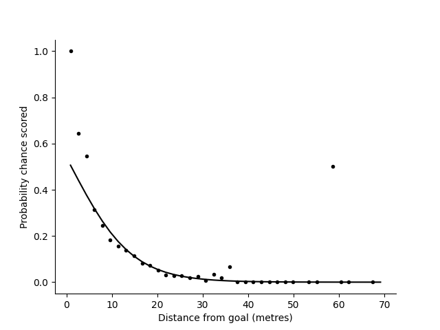
Investigating the relationship between probability of scoring goals and distance to goal
We want to find out if the distanse influences the probability of scoring a goal. First we plot the probability of scoring given the distance. Then, we fit logistic regression to the data.
#number of shots
shotcount_dist = np.histogram(shots['Distance'],bins=40,range=[0, 70])
#number of goals
goalcount_dist = np.histogram(goals['Distance'],bins=40,range=[0, 70])
#empirical probability of scoring
prob_goal = np.divide(goalcount_dist[0],shotcount_dist[0])
distance = shotcount_dist[1]
middistance= (distance[:-1] + distance[1:])/2
#making a plot
fig, ax = plt.subplots()
#plotting data
ax.plot(middistance, prob_goal, linestyle='none', marker= '.', color='black')
#making legend
ax.set_ylabel('Probability chance scored')
ax.set_xlabel("Distance from goal (metres)")
ax.spines['top'].set_visible(False)
ax.spines['right'].set_visible(False)


#make single variable model of distance
test_model = smf.glm(formula="Goal ~ Distance" , data=shots,
                           family=sm.families.Binomial()).fit()
#print summary
print(test_model.summary())
b=test_model.params
#calculate xG
xGprob=1/(1+np.exp(-(b[0]+b[1]*middistance)))
#plot line
ax.plot(middistance, xGprob, linestyle='solid', color='black')
plt.show()
                 Generalized Linear Model Regression Results
==============================================================================
Dep. Variable:                   Goal   No. Observations:                 8451
Model:                            GLM   Df Residuals:                     8449
Model Family:                Binomial   Df Model:                            1
Link Function:                  Logit   Scale:                          1.0000
Method:                          IRLS   Log-Likelihood:                -2524.4
Date:                Thu, 20 Nov 2025   Deviance:                       5048.9
Time:                        06:56:32   Pearson chi2:                 1.56e+04
No. Iterations:                     6   Pseudo R-squ. (CS):            0.08410
Covariance Type:            nonrobust
==============================================================================
                 coef    std err          z      P>|z|      [0.025      0.975]
------------------------------------------------------------------------------
Intercept      0.1555      0.090      1.732      0.083      -0.020       0.331
Distance      -0.1496      0.006    -23.243      0.000      -0.162      -0.137
==============================================================================
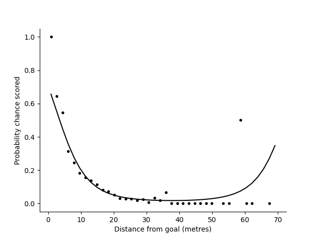
- Adding squared distance to the model
To our model we can add more variables than only one. We can try adding distance to goal squared and see if it improves our predictions.
calculating distance squared
shots["D2"] = shots['Distance']**2
#adding it to the model
test_model = smf.glm(formula="Goal ~ Distance + D2" , data=shots,
                           family=sm.families.Binomial()).fit()
#print model summary
print(test_model.summary())
#get parameters
b=test_model.params
#calculate xG
xGprob=1/(1+np.exp(-(b[0]+b[1]*middistance+b[2]*pow(middistance,2))))
fig, ax = plt.subplots()
#plot line
ax.plot(middistance, prob_goal, linestyle='none', marker= '.', color='black')
#make legend
ax.set_ylabel('Probability chance scored')
ax.set_xlabel("Distance from goal (metres)")
ax.spines['top'].set_visible(False)
ax.spines['right'].set_visible(False)
ax.plot(middistance, xGprob, linestyle='solid', color='black')
plt.show()
                 Generalized Linear Model Regression Results
==============================================================================
Dep. Variable:                   Goal   No. Observations:                 8451
Model:                            GLM   Df Residuals:                     8448
Model Family:                Binomial   Df Model:                            2
Link Function:                  Logit   Scale:                          1.0000
Method:                          IRLS   Log-Likelihood:                -2505.6
Date:                Thu, 20 Nov 2025   Deviance:                       5011.1
Time:                        06:56:32   Pearson chi2:                 8.44e+03
No. Iterations:                     7   Pseudo R-squ. (CS):            0.08818
Covariance Type:            nonrobust
==============================================================================
                 coef    std err          z      P>|z|      [0.025      0.975]
------------------------------------------------------------------------------
Intercept      0.8705      0.132      6.618      0.000       0.613       1.128
Distance      -0.2591      0.016    -16.482      0.000      -0.290      -0.228
D2             0.0034      0.000      8.262      0.000       0.003       0.004
==============================================================================
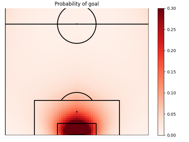
Adding squared distance to the model
To our model we can add more variables than only one. We can try adding distance to goal squared and see if it improves our predictions.
#creating extra variables
shots["X2"] = shots['X']**2
shots["C2"] = shots['C']**2
shots["AX"]  = shots['Angle']*shots['X']

# list the model variables you want here
model_variables = ['Angle','Distance','X','C', "X2", "C2", "AX"]
model=''
for v in model_variables[:-1]:
    model = model  + v + ' + '
model = model + model_variables[-1]

#fit the model
test_model = smf.glm(formula="Goal ~ " + model, data=shots,
                           family=sm.families.Binomial()).fit()
#print summary
print(test_model.summary())
b=test_model.params

#return xG value for more general model
def calculate_xG(sh):
   bsum=b[0]
   for i,v in enumerate(model_variables):
       bsum=bsum+b[i+1]*sh[v]
   xG = 1/(1+np.exp(-bsum))
   return xG

#add an xG to my dataframe
xG=shots.apply(calculate_xG, axis=1)
shots = shots.assign(xG=xG)

#Create a 2D map of xG
pgoal_2d=np.zeros((68,68))
for x in range(68):
    for y in range(68):
        sh=dict()
        a = np.arctan(7.32 *x /(x**2 + abs(y-68/2)**2 - (7.32/2)**2))
        if a<0:
            a = np.pi + a
        sh['Angle'] = a
        sh['Distance'] = np.sqrt(x**2 + abs(y-68/2)**2)
        sh['D2'] = x**2 + abs(y-68/2)**2
        sh['X'] = x
        sh['AX'] = x*a
        sh['X2'] = x**2
        sh['C'] = abs(y-68/2)
        sh['C2'] = (y-68/2)**2

        pgoal_2d[x,y] =  calculate_xG(sh)

#plot pitch
pitch = VerticalPitch(line_color='black', half = True, pitch_type='custom', pitch_length=105, pitch_width=68, line_zorder = 2)
fig, ax = pitch.draw()
#plot probability
pos = ax.imshow(pgoal_2d, extent=[-1,68,68,-1], aspect='auto',cmap=plt.cm.Reds,vmin=0, vmax=0.3, zorder = 1)
fig.colorbar(pos, ax=ax)
#make legend
ax.set_title('Probability of goal')
plt.xlim((0,68))
plt.ylim((0,60))
plt.gca().set_aspect('equal', adjustable='box')
plt.show()
                 Generalized Linear Model Regression Results
==============================================================================
Dep. Variable:                   Goal   No. Observations:                 8451
Model:                            GLM   Df Residuals:                     8443
Model Family:                Binomial   Df Model:                            7
Link Function:                  Logit   Scale:                          1.0000
Method:                          IRLS   Log-Likelihood:                -2498.7
Date:                Thu, 20 Nov 2025   Deviance:                       4997.4
Time:                        06:56:33   Pearson chi2:                 8.40e+03
No. Iterations:                     7   Pseudo R-squ. (CS):            0.08966
Covariance Type:            nonrobust
==============================================================================
                 coef    std err          z      P>|z|      [0.025      0.975]
------------------------------------------------------------------------------
Intercept      0.5103      0.887      0.576      0.565      -1.228       2.248
Angle          0.6338      0.319      1.989      0.047       0.009       1.258
Distance      -0.2798      0.118     -2.381      0.017      -0.510      -0.049
X              0.1243      0.124      1.001      0.317      -0.119       0.368
C             -0.0300      0.040     -0.750      0.454      -0.109       0.048
X2             0.0014      0.001      1.422      0.155      -0.001       0.003
C2             0.0041      0.003      1.398      0.162      -0.002       0.010
AX            -0.1251      0.118     -1.063      0.288      -0.356       0.105
==============================================================================
Testing model fit
Every time we make a model, it is important to test it. We test our logistic regression model using Mcfaddens Rsquared and ROC curve.
# Mcfaddens Rsquared for Logistic regression
null_model = smf.glm(formula="Goal ~ 1 ", data=shots,
                     family=sm.families.Binomial()).fit()
print("Mcfaddens Rsquared", 1 - test_model.llf / null_model.llf)

# ROC curve
numobs = 100
TP = np.zeros(numobs)
FP = np.zeros(numobs)
TN = np.zeros(numobs)
FN = np.zeros(numobs)

for i, threshold in enumerate(np.arange(0, 1, 1 / numobs)):
    for j, shot in shots.iterrows():
        if (shot['Goal'] == 1):
            if (shot['xG'] > threshold):
                TP[i] = TP[i] + 1
            else:
                FN[i] = FN[i] + 1
        if (shot['Goal'] == 0):
            if (shot['xG'] > threshold):
                FP[i] = FP[i] + 1
            else:
                TN[i] = TN[i] + 1

fig, ax = plt.subplots()
ax.plot(FP / (FP + TN), TP / (TP + FN), color='black')
ax.plot([0, 1], [0, 1], linestyle='dotted', color='black')
ax.set_ylabel("Predicted to score and did TP/(TP+FN))")
ax.set_xlabel("Predicted to score but didn't FP/(FP+TN)")
plt.ylim((0.00, 1.00))
plt.xlim((0.00, 1.00))
ax.spines['top'].set_visible(False)
ax.spines['right'].set_visible(False)
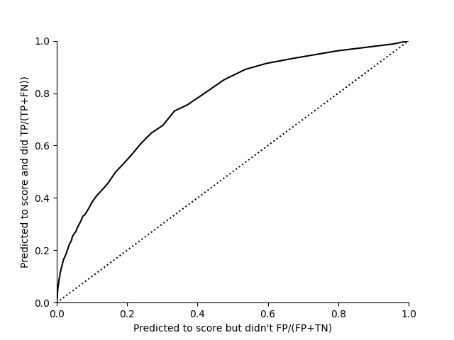
Mcfaddens Rsquared 0.13708006325049105
Challenge
Create different models for headers and non-headers (as suggested in Measuring the Effectiveness of Playing Strategies at Soccer, Pollard (1997))!
Assign to penalties xG = 0.8!
Find out which player had the highest xG in 2017/18 Premier League season!
Total running time of the script: ( 0 minutes 25.636 seconds)