Making Voronoi Diagrams

Making Voronoi Diagrams with Statsbomb 360 data

from mplsoccer import Sbopen, VerticalPitch
import numpy as np
import matplotlib.pyplot as plt
# The first thing we have to do is open the data. We use a parser SBopen available in mplsoccer.

Opening data

For this task we will use Statsbomb 360 data form Sweden against Switzerland game at the Women’s UEFA Euro 2022. We want to make the plot for Bennison’s goal from that game. We also take the id of this event. As the next step we open the 360 data. In df_frame player location is stored and in df_visible area tracked by Statsbomb during this event. From the latter we take visible area only for this specific event and store it as a numpy array with apeces coordinates stored in separate rows.

#declare mplsoccer parser
parser = Sbopen()

#open event dataset
df_event = parser.event(3835331)[0]
#find Bennison goal
event = df_event.loc[df_event["outcome_name"] == 'Goal'].loc[df_event["player_name"] == 'Hanna Ulrika Bennison']
#save it's id
event_id = event["id"].iloc[0]

#open 360
df_frame, df_visible = parser.frame(3835331)
#get visible area
visible_area = np.array(df_visible.loc[df_visible["id"] == event_id]['visible_area'].iloc[0]).reshape(-1, 2)

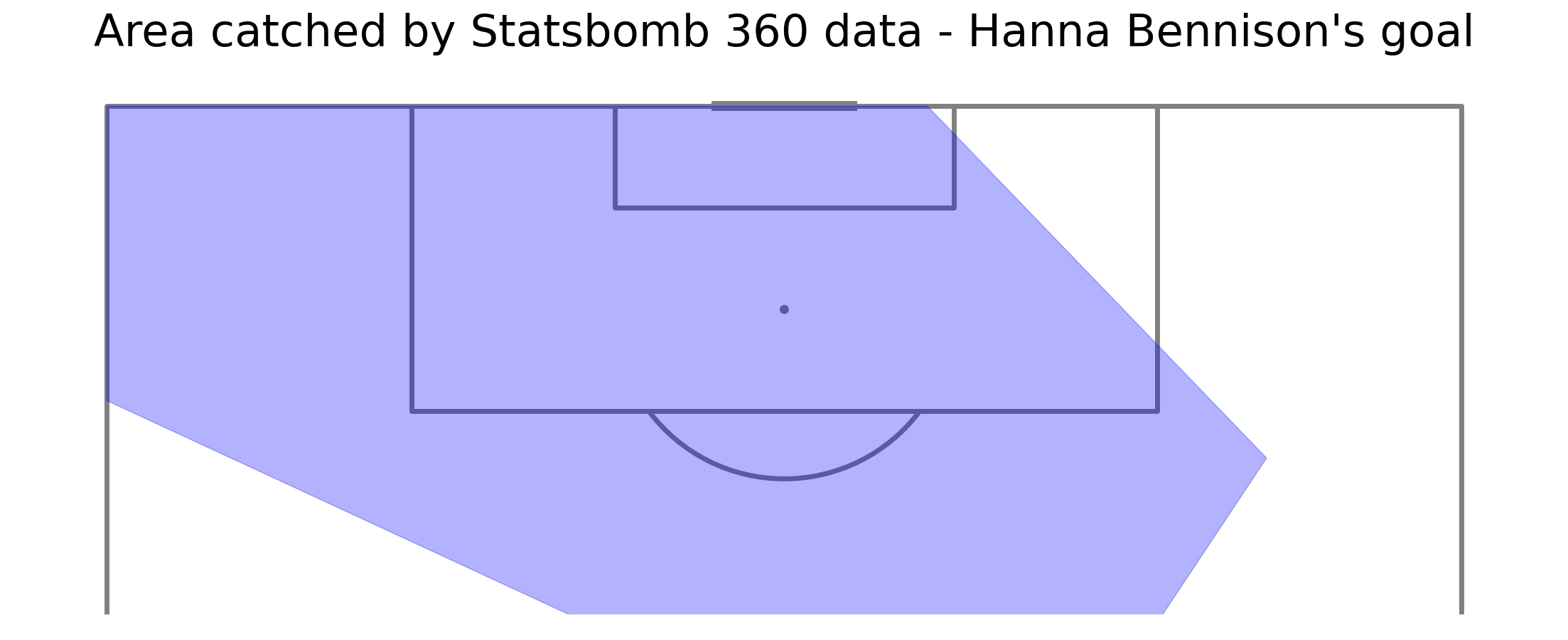
Plotting visible area

To investigate the area that Statsbomb managed to catch, we plot it using polygon method of mplsoccer.

pitch  = VerticalPitch(line_color='grey', line_zorder = 1, half = True, pad_bottom=-30, linewidth=5)
fig, ax = pitch.grid(grid_height=0.9, title_height=0.06, axis=False,
                     endnote_height=0.04, title_space=0, endnote_space=0)
#add visible area
pitch.polygon([visible_area], color=(0, 0, 1, 0.3), ax=ax["pitch"], zorder = 2)
fig.suptitle("Area catched by Statsbomb 360 data - Hanna Bennison's goal", fontsize = 45)
plt.show()

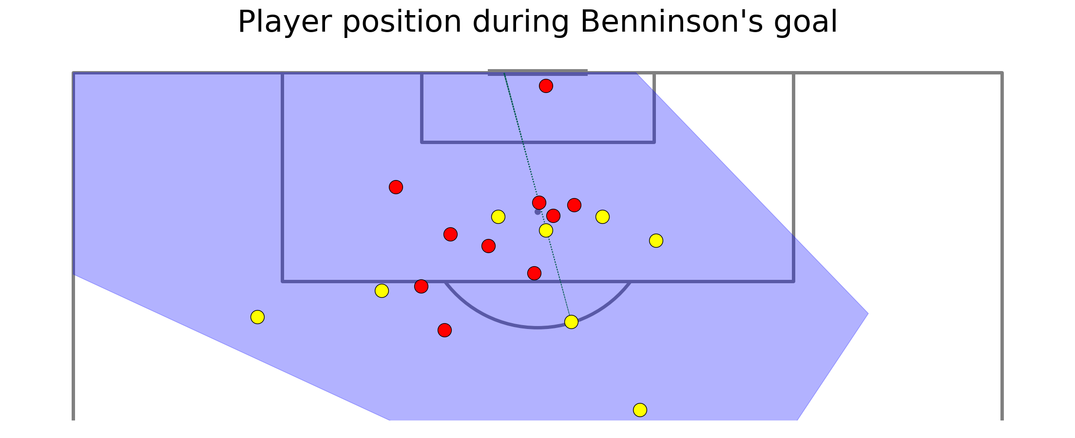
Plotting player position

Now, to get a better understanding of Statsbomb 360 data, we can plot player position during the shot as well as shot trajectory.

#get player position for this event
player_position = df_frame.loc[df_frame["id"] == event_id]
#get swedish player position
sweden = player_position.loc[player_position["teammate"] == True]
#get swiss player positions
swiss = player_position.loc[player_position["teammate"] == False]

fig, ax = pitch.grid(grid_height=0.9, title_height=0.06, axis=False,
                     endnote_height=0.04, title_space=0, endnote_space=0)
#plot visible area
pitch.polygon([visible_area], color=(0, 0, 1, 0.3), ax=ax["pitch"], zorder = 2)
#plot sweden players - yellow
pitch.scatter(sweden.x, sweden.y, color = 'yellow', edgecolors = 'black', s = 400, ax=ax['pitch'], zorder = 3)
#plot swiss players - red
pitch.scatter(swiss.x, swiss.y, color = 'red', edgecolors = 'black', s = 400, ax=ax['pitch'], zorder = 3)
#add shot
pitch.lines(event.x, event.y,
                   event.end_x, event.end_y, comet = True, color='green', ax=ax['pitch'], zorder = 1, linestyle = ':', lw = 2)
fig.suptitle("Player position during Benninson's goal", fontsize = 45)
plt.show()

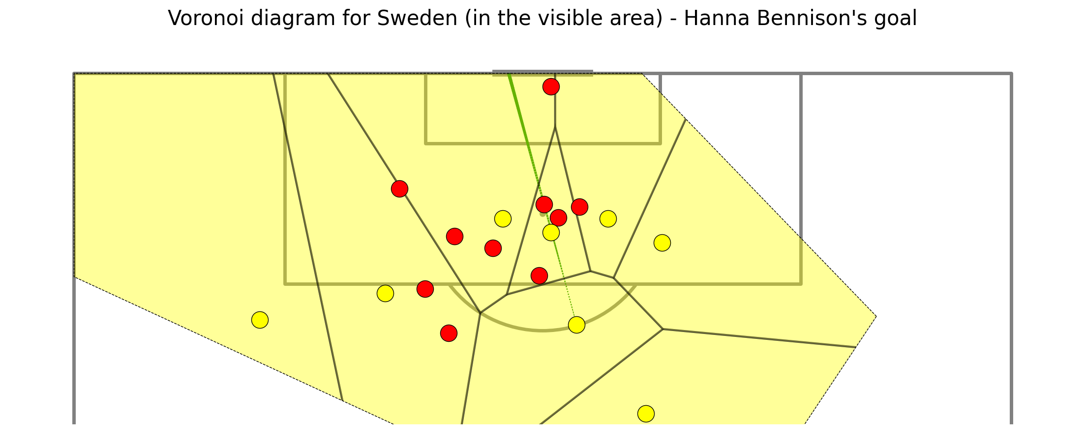
Plotting Voronoi diagrams for 1 team.

Now, we can make Voronoi diagrams for Swedish teams. We do it using voronoi method. Then, we clip the diagram to restricted area only.

#Voronoi for Sweden
team1, team2 = pitch.voronoi(sweden.x, sweden.y,
                         sweden.teammate)
fig, ax = pitch.grid(grid_height=0.9, title_height=0.06, axis=False,
                     endnote_height=0.04, title_space=0, endnote_space=0)
#plot voronoi diagrams as polygons
t1 = pitch.polygon(team1, ax = ax["pitch"], color = 'yellow', ec = 'black', lw=3, alpha=0.4, zorder = 2)
#mark visible area
visible = pitch.polygon([visible_area], color = 'None', linestyle = "--", ec = "black", ax=ax["pitch"], zorder = 2)
#plot swedish players
pitch.scatter(sweden.x, sweden.y, color = 'yellow', edgecolors = 'black', s = 600, ax=ax['pitch'], zorder = 4)
#plot swiss players
pitch.scatter(swiss.x, swiss.y, color = 'red', edgecolors = 'black', s = 600, ax=ax['pitch'], zorder = 3)
#plot shot
pitch.lines(event.x, event.y,
                   event.end_x, event.end_y, comet = True, color='green', ax=ax['pitch'], zorder = 1, linestyle = ':', lw = 5)
#limit voronoi diagram to polygon
for p1 in t1:
    p1.set_clip_path(visible[0])
fig.suptitle("Voronoi diagram for Sweden (in the visible area) - Hanna Bennison's goal", fontsize = 30)
plt.show()

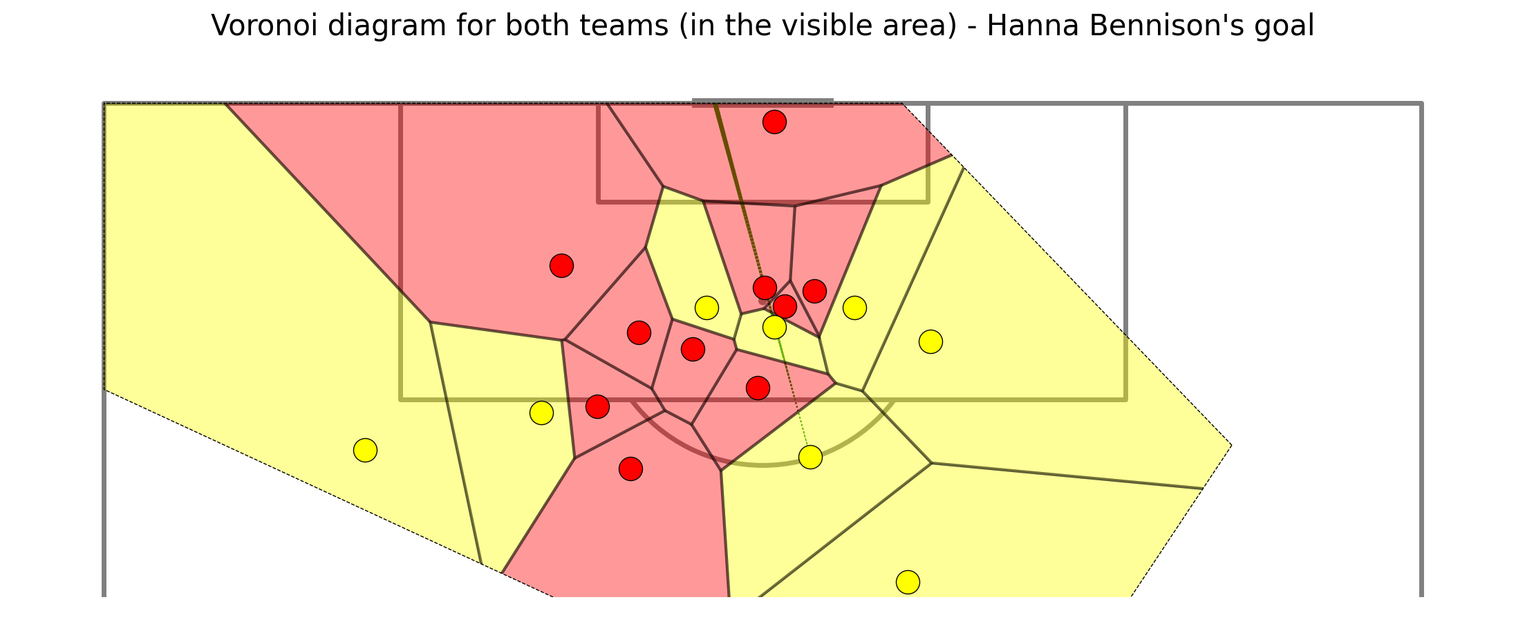
Plotting Voronoi diagrams for 2 teams.

We can also differentiate between areas and mark areas that each player was the closest to. To do that instead of using a dataframe with only one team players’ position, we use both teams.

#voronoi for both teams
team1, team2 = pitch.voronoi(player_position.x, player_position.y,
                         player_position.teammate)
fig, ax = pitch.grid(grid_height=0.9, title_height=0.06, axis=False,
                     endnote_height=0.04, title_space=0, endnote_space=0)
#add sweden
t1 = pitch.polygon(team1, ax = ax["pitch"], color = 'yellow', ec = 'black', lw=3, alpha=0.4, zorder = 2)
#add switzerland
t2 = pitch.polygon(team2, ax = ax["pitch"], color = 'red', ec = 'black', lw=3, alpha=0.4, zorder = 2)
#mark visible area
visible = pitch.polygon([visible_area], color = 'None', linestyle = "--", ec = "black", ax=ax["pitch"], zorder = 2)
#plot swedish players
pitch.scatter(sweden.x, sweden.y, color = 'yellow', edgecolors = 'black', s = 600, ax=ax['pitch'], zorder = 4)
#plot swiss players
pitch.scatter(swiss.x, swiss.y, color = 'red', edgecolors = 'black', s = 600, ax=ax['pitch'], zorder = 3)
#plot shot
pitch.lines(event.x, event.y,
                   event.end_x, event.end_y, comet = True, color='green', ax=ax['pitch'], zorder = 1, linestyle = ':', lw = 5)
#clip sweden
for p1 in t1:
    p1.set_clip_path(visible[0])
#clip sswitzerland
for p2 in t2:
    p2.set_clip_path(visible[0])
fig.suptitle("Voronoi diagram for both teams (in the visible area) - Hanna Bennison's goal", fontsize = 30)
plt.show()